MathMap Examples

You can find lots of examples of MathMap generated images at the very interesting and well-written page about visualizing complex functions by Hans Lundmark.

Some guys at Stanford have used MathMap to recreate M.C. Escher's "Print Gallery" with a photograph.

Alexander Heide has used MathMap to transform x-ray images of crystals.

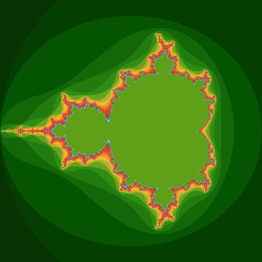
Tom Rathborne has used MathMap to generate some very unusual Mandelbrot fractal images.

Laurent Despeyroux has a page with GIMP tutorials which make use of MathMap to create interesting effects.

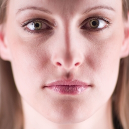
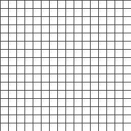
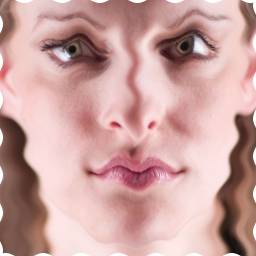
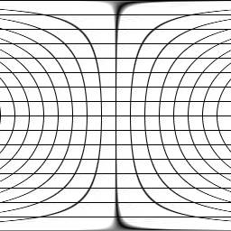
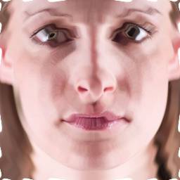
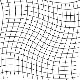
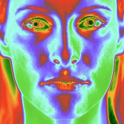
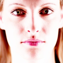
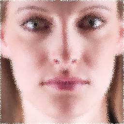
The following are examples of MathMap expressions, together with their effect on two images. Variants of all of these expression are included as examples in the plug-in.

The original images:

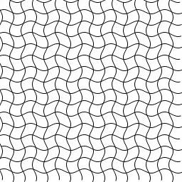
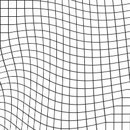
filter wave (image in)
    in(xy+xy:[sin(y/6),sin(x/6)]*3)
end

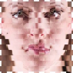
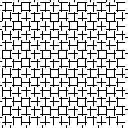
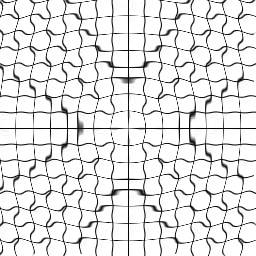
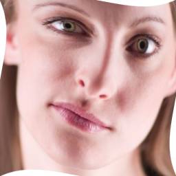
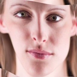
filter slice (image in)
    in(xy+xy:[5*sign(cos(y/6)),5*sign(cos(x/6))])
end

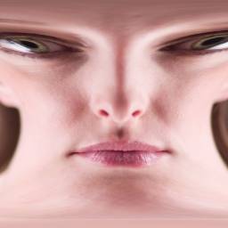
filter mercator (image in)
    in(xy*xy:[cos(pi/2/Y*y),1])
end

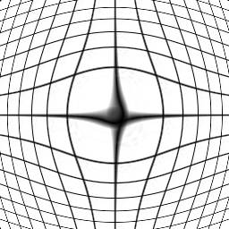
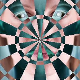
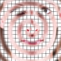
filter pond (image in)
    in(ra+ra:[sin(r/3)*3,0])
end

filter twirl (image in)
    in(ra+ra:[0,-(r/R-1)*pi/5])
end

filter jitter (image in)
    in(ra:[r,a+a%0.14-0.07])
end

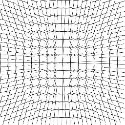
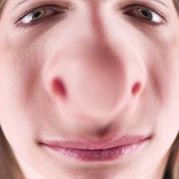
filter fisheye (image in)
    in(ra:[r*r/R,a])
end

The result of this expression depends on the gradient and on the value of t.

filter colorify (image in, gradient grad)
    grad((gray(in(xy))+t)%1)
end

The result of this expression depends on the setting of the curve.

filter gamma (image in, curve gamma)
    p=in(xy);
    rgbaColor(gamma(red(p)),gamma(green(p)),gamma(blue(p)),alpha(p))
end

As does this (there are actually two curves here and one slider).

unit filter curve_bend (unit image in, float alpha: 0-6.28318530,
                        curve lower, curve upper)
    dir = xy:[cos(alpha),sin(alpha)];
    ndir = xy:[-dir[1],dir[0]];
    p = xy / m2x2:[dir[0],-ndir[0],
                   dir[1],-ndir[1]];
    pt = dir * p[0];
    vec = xy - pt;
    dist = -p[1];
    pos = 0.5 + p[0] / 2;
    lo = 1 / (lower(pos) * 4 - 2);
    up = 1 / (upper(pos) * 4 - 2);
    f = lo + ((dist + 1) / 2) * (up - lo);
    in(pt + ndir * f)
end

filter scatter (image in)
    in(xy+xy:[rand(-3,3),rand(-3,3)])
end

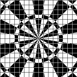
filter darts (image in)
    p=in(xy);
    p=if inintv((a-(pi/20))%(pi/5),0,(pi/10)) then p else -p+1 end;
    if inintv(r%80,68,80) then p else -p+1 end
end

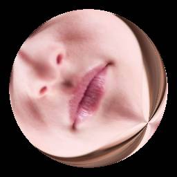
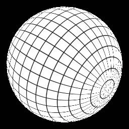
filter sphere (image in)
    # Thanks to Herbert Poetzl
    rd=0.9*min(X,Y);
    if r>rd then
        rgba:[0,0,0,1]
    else
        alpha=-(5/3)*pi; beta=(1/3)*pi; gamma=t*pi*2;
        sa=sin(alpha);
        sb=sin(beta);
        ca=cos(alpha);
        cb=cos(beta);
        theta=a;
        phi=acos(r/rd);
        x0=cos(theta)*cos(phi);
        y0=sin(theta)*cos(phi);
        z0=sin(phi);
        x1=ca*x0+sa*y0;
        z1=-sa*-sb*x0+ca*-sb*y0+cb*z0;
        if z1 >= 0 || 1 then
            y1=cb*-sa*x0+cb*ca*y0+sb*z0
        else
            z1=z1-2*cb*z0;
            y1=cb*-sa*x0+cb*ca*y0-sb*z0
        end;
        theta1=atan(-x1/y1)+(if y1>0 then pi/2 else 3*pi/2 end);
        phi1=asin(z1);
        in(xy:[((theta1*2+gamma)%(pi*2)-pi)/pi*X,-phi1/(pi/2)*Y])
    end
end

This is an example of combining MathMaps alpha operation with layers. The background is the image of Elisa. The second layer is the grid, which has been MathMapped with the following expression:

filter alpha_spiral (image in)
    in(xy)*rgba:[1,1,1,0]+rgba:[0,0,0,sin((r-a*6)/6+t*2*pi)*0.5+0.5]
end

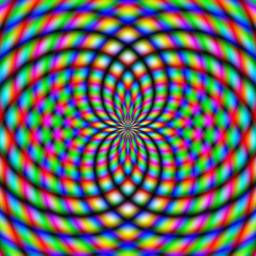
filter moire1 ()
    abs(rgba:[sin(r/4)+sin(15*a),sin(r/3.5)+sin(17*a),sin(r/3)+sin(19*a),2])*0.5
end

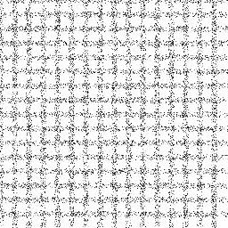
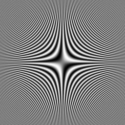
filter moire2 ()
    grayColor(sin(x*y/180*pi)*0.5+0.5)
end

This is a simple Mandelbrot fractal, colorized by a gradient. For more complex Mandelbrot images rendered with MathMap, see Tom Rathborne's page

filter mandelbrot (gradient coloration)
    p=ri:(xy/xy:[X,X]*1.5-xy:[0.5,0]);
    c=ri:[0,0];
    iter=0;
    while abs(c)<2 && iter<31
    do
        c=c*c+p;
        iter=iter+1
    end;
    coloration(iter/32)
end